When Hippasus of Metapontum discovered irrational numbers, he was said to have been cast into the ocean—so unnatural was this concept to the Greeks, the legend goes, that they considered it an affront to the gods. While the historical accuracy of this tale has not been conclusively established[1]
Thompson, William. The Commentary of Pappus on Book X of Euclid's Elements
, Hippasus is generally accepted as an early discoverer of these unnatural numbers. And it all came down to two contradictory tenets of Pythagoreanism—that “all is number”—that is, all lengths are commensurable, and that the pentagram was a sacred shape, to be studied and revered.
What the heretical Hippasus did to earn the ire of his brethren was quite simple—in the center of the pentagram, he drew another pentagram, but upside down. In that pentagram, he drew yet another pentagram, and so on and so forth. He then proved that the pentagrams were shrinking by a factor of the golden ratio each time, and using a geometric argument by the similarity of isosceles triangles, proved that the golden ratio was irrational.[2]
James R. Choike. The Pentagram and the Discovery of an Irrational Number (1980), The Two-Year College Mathematics Journal, 11:5, 312-316
When I was in school, we were taught that he had proved that $\sqrt{2}$ is irrational by dramatically drawing the diagonal of a square in front of a shocked audience. Not sure which story is cooler—probably the pentagram.
The irony in the Pythagoreans’ reaction is obvious to us in retrospect—today, irrational numbers, like pi and the square root of two, are found everywhere in natural processes, from planetary orbits to electron repulsions. We see irrational dimensions in human cells, in branching trees, in flowers...Irrational dimensions, you ask? Well, allow me to be your Hippasus.
When we think about dimension, we often don’t really know what we’re talking about. The only real intuition we have is the world we live in is three-dimensional, and the sheet of paper in front of you, is, to an approximation, two-dimensional. But is it really? On one hand, it’s very thin; on the other hand, it does have some height. What about a spider web? Isn’t made up of one-dimensional lines forming a two-dimensional web? Is it one, two, three, or...maybe...four-dimensional?
To try to answer these questions, let’s first agree on a couple of things—that a line segment is one-dimensional; a square, two-dimensional; a cube, three-dimensional. To dive in deeper, however, we’ll need the same concept that led to Hippasus’ untimely demise—self-similarity."Self-similarity is a dull subject because you are used to very familiar shapes. But that is not the case. Now many shapes which are self-similar again, the same seen from close by and far away, and which are far from being straight or plane or solid." (Benoit Mandelbrot)
Let’s begin with a line segment. Is a line segment self-similar? Well, if I give you two line segments, you can join them end-to-end and make a line segment twice as long. Similarly, you can cut a line segment in half, and make two line segments, twice as short.
What about a square? Given a square of a certain size, it takes four copies of that square to make a larger square—just like if we’d stretched the original in all directions by a factor of two. And what about a cube? It takes eight copies of a cube to make a larger cube, one that’s the size of the original, stretched in all directions by a factor of two.
What’s the point of these observations? Well, in fact, we can use this to define dimension—if it takes $n$ copies of a shape to make the same shape $r$ times as big, we define the dimension of that shape to be $\log_r n$. For instance, the dimension of a square is $\log_2 4 = 2$, since we used four copies and made a square twice as big. Similarly, we get the dimension of a line to be $\log_2 2 = 1$, and a cube is $\log_2 8 = 3$-dimensional.
The beauty of this definition is that it lets us calculate the dimension for what are known as Lindenmayer systems—a process of repeatedly applying a set of rules to a string of characters, invented by Aristid Lindenmayer in 1968 to study plant development.[4]
Grzegorz Rozenberg and Arto Salomaa. The mathematical theory of L systems (1980).
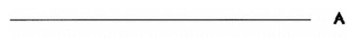
Hmm, plant development! To me, that sounds pretty...natural! A famous L-system is as follows: starting with the letter $\texttt{S}$, apply the following rule: “replace every $\texttt{S}$ with $\texttt{S+S--S+S}$”. So, at the first step, we have $\texttt{S}$; at the second step, we have $\texttt{S+S--S+S}$; at the third step, we have $\texttt{S+S--S+S+S+S--S+S--S+S--S+S+S+S--S+S}$; and so on. These strange symbols have meaning—imagine we’re on an infinite canvas, and we’re the tip of a brush. The $\texttt{S}$ tells us to move forward by a centimeter; the $\texttt{+}$ tells us to turn left 60 degrees, and the $\texttt{-}$ tells us to turn right 60 degrees. Then, step 1 simply describes a line:
$\texttt{S}$.
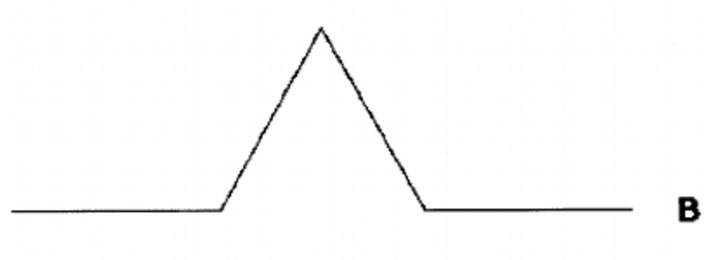
Step 2 is one replacement:
$\texttt{S+S--S+S}$.
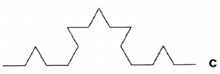
Step 3 looks like this:
$\texttt{S+S--S+S+S+S--S+S--S+S--S+S+S+S--S+S}$.
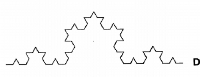
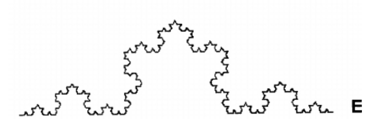
As you may begin to notice, the rule simply tells us to replace every straight line with a spiky line pointing outward, ad infinitum. This is known as the Koch curve, which was invented over a hundred years ago by the Swedish mathematician Helge von Koch. Here’s the question we were building up to—what is the dimension of the Koch curve?
Well, we need four copies of the Koch curve to create another one that’s three times as large—so its dimension is $\log_3 4$, or approximately 1.2619. This makes some intuitive sense—it clearly takes up more space than a line, so it shouldn’t be called one-dimensional; however, it’s not quite as “big” as a plane, so we can’t call it two-dimensional, either. 1.2619? A perfect compromise.
Let’s go back to the Greeks for a second. Say they gave Hippasus one shot—a ten-minute presentation, for instance—to convince them that irrational numbers were “natural”. If he could convince them, he lived. If irrationals remained “unnatural” to the Pythagoreans, he would be fast friends with the ocean floor. Placed in such a situation, it might be unclear to us how a Lindenmayer system might help—after all, the Koch curve above was so perfect, so infinite, that nothing of the sort could ever show up in nature.
But what if we made it less perfect?
Say that, at every step, instead of blindly applying the rule $\texttt{S} \rightarrow \texttt{S+S--S+S}$, we flip a coin—if it’s heads, we replace that $\texttt{S}$ with $\texttt{S+S--S+S}$; if it’s tails, we replace $\texttt{S}$ with $\texttt{S-S++S-S}$. That is, roughly half of our replacements will stick outward, like usual; however, half of them will stick inward. This shape starts to look as follows:
Starting to look a bit more "natural", isn’t it? Since everything is being generated live in the browser, try chancing the probability for yourself:
50%
We can show with some simple tricks that this “strange” Koch curve has the same dimension as the normal one—still an irrational number. You tell this to the Greeks, but they’re still not convinced. They look at the curve, and say, “what in nature looks like this? The trees, the grass?” Your protestation that “you once saw an island like that” makes them reach for the ropes.
All right, let’s save you from the angry Pythagoreans. Start with the letter $\texttt{X}$, and replace each $\texttt{X}$ with $\texttt{F+[[X]-X]-F[-FX]+X}$, and each $\texttt{F}$ with $\texttt{FF}$. Here $\texttt{F}$ means go straight; $\texttt{-}$ and $\texttt{+}$ mean turn left and right by 25 degrees; and things done in brackets are forgotten after they’re done. In the five minutes you have left, you draw this $1.4523...$-dimensional system for $n=6$:
The Pythagoreans, of course, are going to immediately ask you to determine the dimensions of all the trees around them. Don't fret—Zhang, Dongsheng; Samal, Ashok; and Brandle, James R., A Method for Estimating Fractal Dimension of Tree Crowns from Digital Images (2007) has you covered. The average Japanese yew, as it turns out, is fully 2.45-dimensional, while the eastern white pine is a mere 2.24-dimensional tree. According to their paper, "The smaller value of fractal dimension indicates that the foliage of the tree crown is located on the crown periphery and its mass and surface are proportional to the surface of the convex hull. On the other hand, a large value of fractal dimension implies that foliage was uniformly distributed throughout the crown volume". So if the Greeks point out a tree with dense uniform leaves, guess closer to 3-dimensional; if the leaves are on the periphery, well, that's almost a 2-dimensional tree. More fun facts: the coastline of Ireland is roughly 1.22-dimensional, whereas that of Great Britain is 1.25-D, and Norway is 1.52-D. Cauiliflower is higher dimension that most trees at 2.8, and the human lung is 2.97-dimensional. (Source: List of fractals by Hausdorff dimension)
Ok, so, you've shown the Pythagoreans a way to create complex, natural beings—of irrational dimension—from a very simple set of repeatedly-applied rules. However, from the back of the crowd, a farmer cries out, "what use is this? I'm no artist, I don't have a computer[6]
In fact, modern computer graphics artists often use Lindenmayer systems to generate realistic tree structures for animated films! However, unless you're the brilliant Thomasina Coverly from Arcadia (which is the best play ever written), you probably won't write out thousands of iterations of these rules by hand.
—if, as you say, a couple simple rules can describe nature, surely I should be able to make use of them!"
At this point, you're tired of the constant life-and-death interrogation from the educated elites, so you tell the farmer—give me a job on your farm for a couple of years, and I'll tell you all about the mathematical laws of nature. The farmer agrees, and you spend five years growing barley together. However, despite barley's status in Metapontum as the symbol of wealth[7]
Carter, Joseph Coleman, ed. Living off the Chora: Diet and Nutrition at Metaponto (2003)
, you simply can't get rich. One thing is stopping you from making a living—the barley earworm keeps destroying your crops! Unable to leave your scientific instincts behind, you decide to count the number of these pests that you can find in a representative square foot of your field. Year over year, you get the following results:
Year 1
69 worms
Year 2
85 worms
Year 3
51 worms
Year 4
99 worms
Oh no! It sure looks like the worms are taking over your turf. You go out to buy pesticides, only to find the hardware store’s shelves empty—it's, like, 2000BC, and besides, pesticides before 1850 weren't awfully effective[8]
Unsworth, John. History of Pesticide Use (2010).
. Distraught, you realize that your next year’s harvest will likely be destroyed as well—and with it, your reputation as a decent farmhand. So, when next year comes, as you go out to weep about your barren fields, something strange happens—lush ears of barley are overflowing their stocks, succulent and golden. You count the number of earworms—there are only five to be seen! Has a miracle happened? Will the pests be gone forever? The answers are no and no—all due to the magic of dynamical systems.
What is a dynamical system? In essence, anything that changes itself according to a rule. For instance, the positions of water molecules in a pipe change by the laws of fluid dynamics; the populations of corn earworms change by the laws of population dynamics—so, these are all dynamical systems.[9]
This may be an awfully broad definition, but that’s sort of by design—for instance, if we can prove something about a general dynamical system, we can apply it to hundreds of others!
More rigorously, a dynamical system is a set—the positions molecules can take on in a pipe of water, the potential sizes a population of earworms can have, etc—and a map that shows us how to get from one state to the next. For instance, given the population this year, what will the population next year be? Note that a system is not a dynamical system if the maps don’t go from the set to itself—for instance, if our set was whole numbers, and our map was division by two, we’d be in a lot of trouble since 14 would go to 7, and 7 would go to 3.5, and 3.5 would go to...nowhere. You get the point.
To get some more intuition, let’s look at one of the simplest possible systems—the logistic map. Created by Pierre François Verhulst in the 19th century,[11]
TVerhulst, P.-F. Recherches mathématiques sur la loi d'accroissement de la population. Nouv. mém. de l'Academie Royale des Sci. et Belles-Lettres de Bruxelles 18, 1-41, 1845.
it aims to describe population growth using two assumptions—when a population is small, it tends to grow exponentially; however, when it becomes too big for the environment to sustain, growth slows down, and the population may contract. That is, if the current population is $x$ percent of the maximum the environment can sustain, the population next year will be $$rx \left(1 - x\right) \text{.}$$
Note that when $x$ is small, the $1-x$ term makes the population grow pretty fast; conversely, when $x$ is large, the $1-x$ term brings the growth rate close to zero. The parameter $r$ is known as the logistic parameter, which basically determines what happens to the population. For instance, when $r<1$, the population dies out:
but when r is between 1 and 3, the population stabilizes:
That is, it doesn’t significantly change year-over-year—the number of animals dying exactly equals the number of births—this is what we call a stable dynamic equilibrium. However, most interesting behaviour tends to happen when $r$ is even larger than that—for instance, what do the population dynamics look like when $r=3$?
Now this is starting to look more interesting. If a species of insect reproduces too fast, we see a biennial boom-bust cycle: too many insects leads to severe competition for resources, so not many eggs are laid; however, the smaller amount of children have abundant resources to themselves, giving birth to many offspring, and the cycle continues. If we increase $r$ even further, we get an even more interesting pattern:
After an initial stabilization, each population cycle now spans a four-year period! If we increase $r$ even further—to 3.55, for instance—the population cycles will now span an eight-year period.[12]
This is known as a period-doubling bifurcation—in fact, Li and Yorke proved in a 1975 paper that for any given period length in years, there exists a value of $r$ that gets you that period! (Tien-Yien Li; James A. Yorke. Period Three Implies Chaos, The American Mathematical Monthly, Vol. 82, No. 10. (Dec., 1975), pp. 985-992.)
However, if we increase $r$ to any value past 3.6, we get a terrifying result—
total unpredictability. The observant reader will object to my use of this term—surely the map is deterministic, so if we know the initial conditions, we can predict the population any number of years from now. To this, I will counter by inviting the reader to look again at the previous diagram.
In this chart, you see the behaviour of the dynamical system for $r=3.9545$. Hover over the values starting at year 6—they’re 0.69, 0.85, 0.51, 0.99, and 0.05. A miracle! You’ve found the exact dynamical system that describes your farm; from now on, you will always know now many worms you’ll have, and you’ll save a fortune by not buying unneeded pesticides! But, how did you find this precise pattern? Let’s say you know the exact logistic parameter for worms on your farm—it’s 3.9545, as above. However, the chart has an initial condition—the original population value—of $x=0.4$. What would happen if that value were changed by a tiny bit—to $x=0.39$?This is one of the central tenets of chaos theory—the exact past predicts the exact future, but the approximate past tells us nothing about the approximate future. Try changing the starting value in this interactive chart:
What’s the takeaway from this example, and what does it mean for us? In fact, this function was popularized in Robert M. May’s seminal paper “Simple mathematical models with very complicated dynamics”[14]
May, R. Simple mathematical models with very complicated dynamics. Nature 261, 459–467 (1976). https://doi.org/10.1038/261459a0
, where he showed that the logistic map and its variants describe dozens of phenomena in physics, economics, and even the social sciences. There are two main things this means for us—that incredibly complex systems can often be described by very simple equations and, conversely, that very simple and stable equations may be the reason we all suddenly die.
If that sounds far-fetched, consider perhaps the most famous dynamical system of all time, and one the ancient Greeks concerned themselves with extensively—the Solar system. We can describe the motion of all nine planets[15]
fight me
as one point in twenty-seven-dimensional space—the first three dimensions are the coordinates of Mercury, the next three dimensions are the coordinates of Venus, the next three are the coordinates of Earth, and so on. Thus, there is a point in this space for any arrangement of the planets. We can use Newton’s Law of Universal Gravitation to derive a map which takes in a given point—the location of all the planets—and outputs another point, say, their location one second in the future. Horrifyingly, despite its simple rules and millions of years of stability, this dynamical system is just as unpredictable as our previous example. Nobody knows this better than Jacques Laskar—in 1989, he showed that Earth’s orbit is chaotic, and a mere fifteen-meter difference in the Earth’s location now leads to absolute unpredictability 100 million years into the future.[16]
Laskar, J. A numerical experiment on the chaotic behaviour of the Solar System. Nature 338, 237–238 (1989). https://doi.org/10.1038/338237a0
The most spectacular result, however, was from Laskar and Gatineau’s 2009 paper—if the orbit of Mercury shifts by just one meter, that is enough to make Mars collide with Earth.[17]
Laskar, J.; Gastineau, M. Existence of collisional trajectories of Mercury, Mars and Venus with the Earth (2009).
Batygin, K., Morbidelli, A. and Holman, M. J. Chaotic Disintegration of the Inner Solar System (2015).
This is the awesome power of dynamical systems—they can be simpler than ever, but still describe the most complex interactions known to us in nature. So the next time you count an unpredictable number of earworms on your farm—make sure Mars is still small in the sky.
If you'd like to cite this article, you can use this:
@misc{gritsevskiy2020nature,
  author = {Gritsevskiy, Andrew},
  title = {The Language of Nature},
  year = {2020},
  howpublished = {Blog post},
  url = {https://andrew.fi/stories/nature/}
}